Page 162 - Genetics_From_Genes_to_Genomes_6th_FULL_Part1

154 Chapter 5 Linkage, Recombination, and the Mapping of Genes on Chromosomes

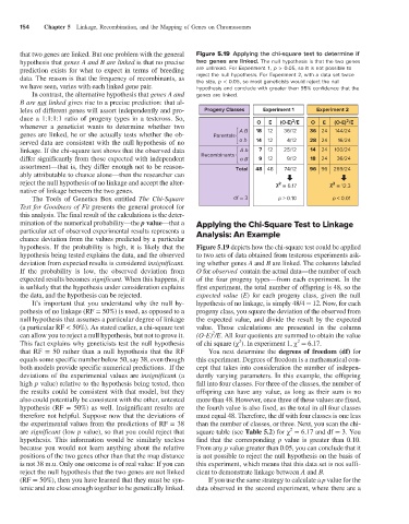
that two genes are linked. But one problem with the general Figure 5.19 Applying the chi-square test to determine if
hypothesis that genes A and B are linked is that no precise two genes are linked. The null hypothesis is that the two genes
prediction exists for what to expect in terms of breeding are unlinked. For Experiment 1, p > 0.05, so it is not possible to
data. The reason is that the frequency of recombinants, as reject the null hypothesis. For Experiment 2, with a data set twice
the size, p < 0.05, so most geneticists would reject the null
we have seen, varies with each linked gene pair. hypothesis and conclude with greater than 95% confidence that the
In contrast, the alternative hypothesis that genes A and genes are linked.
B are not linked gives rise to a precise prediction: that al-
leles of different genes will assort independently and pro- Progeny Classes Experiment 1 Experiment 2
duce a 1:1:1:1 ratio of progeny types in a testcross. So, 2 2
whenever a geneticist wants to determine whether two O E (O-E) /E O E (O-E) /E
genes are linked, he or she actually tests whether the ob- Parentals A B 18 12 36/12 36 24 144/24
served data are consistent with the null hypothesis of no a b 14 12 4/12 28 24 16/24
linkage. If the chi-square test shows that the observed data A b 7 12 25/12 14 24 100/24
differ significantly from those expected with independent Recombinants a B 9 12 9/12 18 24 36/24
assortment—that is, they differ enough not to be reason- Total 48 48 74/12 96 96 269/24
ably attributable to chance alone—then the researcher can
reject the null hypothesis of no linkage and accept the alter- = 6.17 = 12.3
2
2
native of linkage between the two genes.
The Tools of Genetics Box entitled The Chi-Square df = 3 p > 0.10 p < 0.01
Test for Goodness of Fit presents the general protocol for
this analysis. The final result of the calculations is the deter-
mination of the numerical probability—the p value—that a Applying the Chi-Square Test to Linkage
particular set of observed experimental results represents a Analysis: An Example
chance deviation from the values predicted by a particular
hypothesis. If the probability is high, it is likely that the Figure 5.19 depicts how the chi-square test could be applied
hypothesis being tested explains the data, and the observed to two sets of data obtained from testcross experiments ask-
deviation from expected results is considered insignificant. ing whether genes A and B are linked. The columns labeled
If the probability is low, the observed deviation from O for observed contain the actual data—the number of each
expected results becomes significant. When this happens, it of the four progeny types—from each experiment. In the
is unlikely that the hypothesis under consideration explains first experiment, the total number of offspring is 48, so the
the data, and the hypothesis can be rejected. expected value (E) for each progeny class, given the null
It’s important that you understand why the null hy- hypothesis of no linkage, is simply 48/4 = 12. Now, for each
pothesis of no linkage (RF = 50%) is used, as opposed to a progeny class, you square the deviation of the observed from
null hypothesis that assumes a particular degree of linkage the expected value, and divide the result by the expected
(a particular RF < 50%). As stated earlier, a chi-square test value. Those calculations are presented in the column
can allow you to reject a null hypothesis, but not to prove it. (O-E) /E. All four quotients are summed to obtain the value
2
2
2
This fact explains why geneticists test the null hypothesis of chi square (χ ). In experiment 1, χ = 6.17.
that RF = 50 rather than a null hypothesis that the RF You next determine the degrees of freedom (df) for
equals some specific number below 50, say 38, even though this experiment. Degrees of freedom is a mathematical con-
both models provide specific numerical predictions. If the cept that takes into consideration the number of indepen-
deviations of the experimental values are insignificant (a dently varying parameters. In this example, the offspring
high p value) relative to the hypothesis being tested, then fall into four classes. For three of the classes, the number of
the results could be consistent with that model, but they offspring can have any value, as long as their sum is no
also could potentially be consistent with the other, untested more than 48. However, once three of these values are fixed,
hypothesis (RF = 50%) as well. Insignificant results are the fourth value is also fixed, as the total in all four classes
therefore not helpful. Suppose now that the deviations of must equal 48. Therefore, the df with four classes is one less
the experimental values from the predictions of RF = 38 than the number of classes, or three. Next, you scan the chi-
2
are significant (low p value), so that you could reject that square table (see Table 5.2) for χ = 6.17 and df = 3. You
hypothesis. This information would be similarly useless find that the corresponding p value is greater than 0.10.
because you would not learn anything about the relative From any p value greater than 0.05, you can conclude that it
positions of the two genes other than that the map distance is not possible to reject the null hypothesis on the basis of
is not 38 m.u. Only one outcome is of real value: If you can this experiment, which means that this data set is not suffi-
reject the null hypothesis that the two genes are not linked cient to demonstrate linkage between A and B.
(RF = 50%), then you have learned that they must be syn- If you use the same strategy to calculate a p value for the
tenic and are close enough together to be genetically linked. data observed in the second experiment, where there are a